Introduction
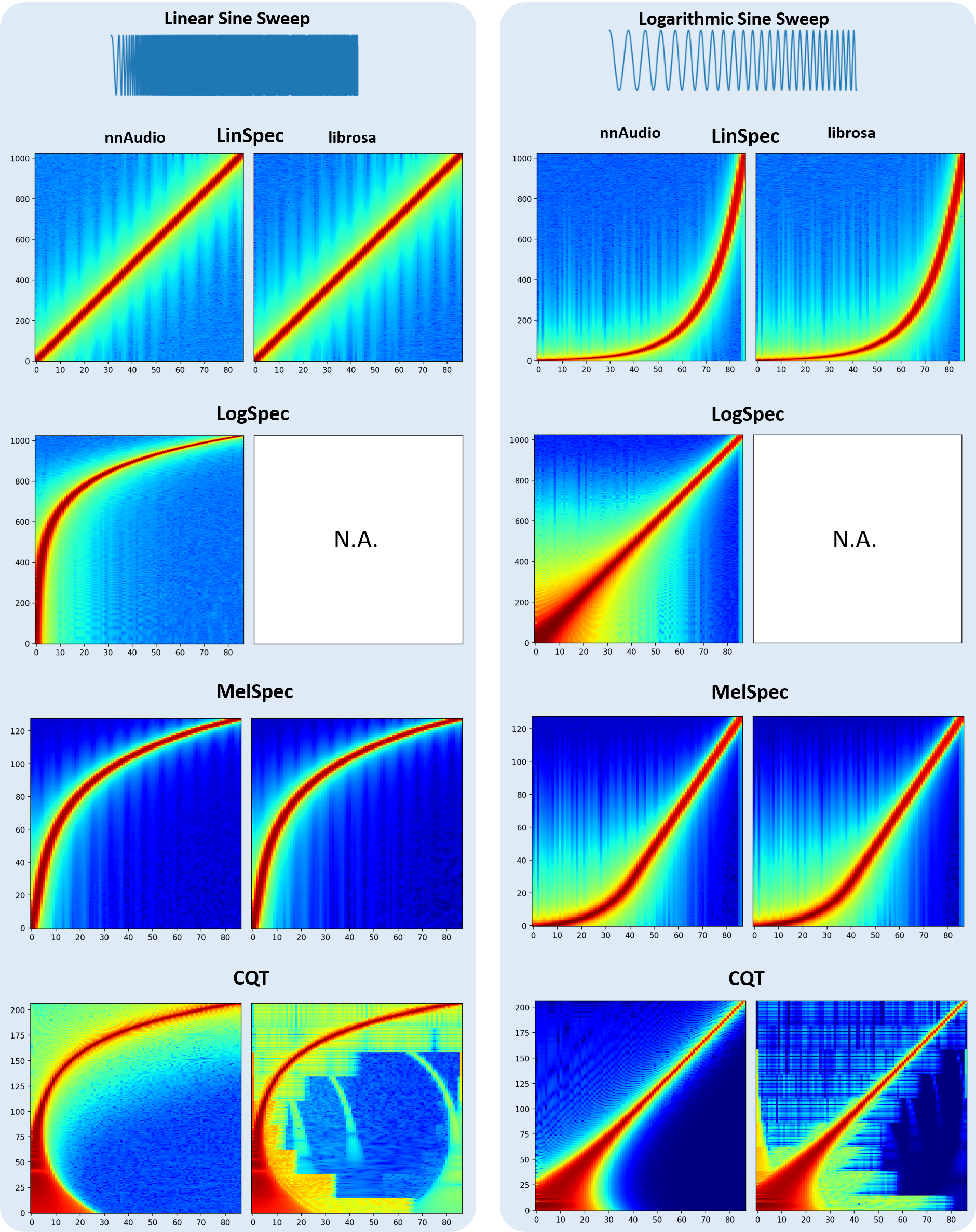
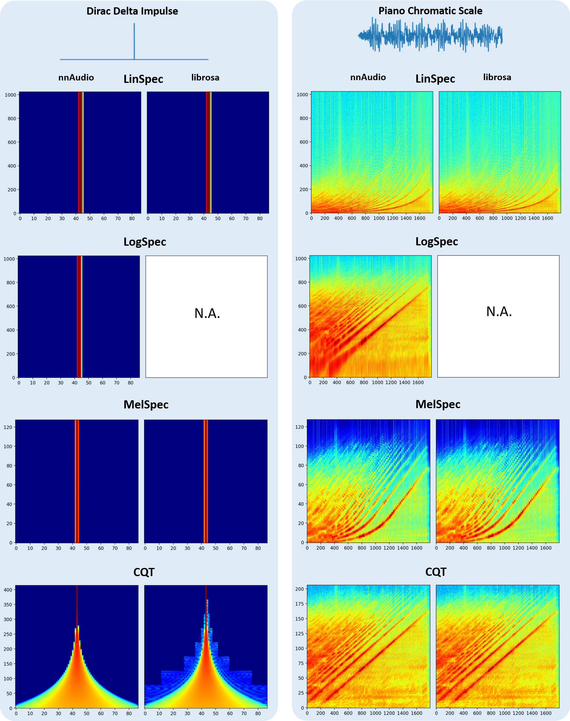
nnAudio is basically a GPU version of some of the librosa functions, with additional features such as differentiable and trainable. The figure below shows the spectrograms obtained by nnAudio and librosa using different input signals.
Installation
Via PyPI
To install previous releases from pypi: pip install nnAudio==x.x.x, where x.x.x is the version number.
The lastest version might not be always available in PyPI, in this case, please install the lastest version from github.
Via GitHub
To install the lastest version from github, you can do pip install git+https://github.com/KinWaiCheuk/nnAudio.git#subdirectory=Installation.
Alternatively, you can also install from the github manually by the following steps:
Clone the repository with
git clone https://github.com/KinWaiCheuk/nnAudio.git <any path you want to save to>cdinto theInstallationfolder where thesetup.pyis located atpython setup.py install.
Requirement
Numpy >= 1.14.5
Scipy >= 1.2.0
PyTorch >= 1.6.0 (Griffin-Lim only available after 1.6.0)
Python >= 3.6
librosa = 0.7.0 (Theortically nnAudio depends on librosa. But we only need to use a single function mel from librosa.filters. To save users troubles from installing librosa for this single function, I just copy the chunk of functions corresponding to mel in my code so that nnAudio runs without the need to install librosa)
Usage
Standalone Usage
To use nnAudio, you need to define the spectrogram layer in the same way as a neural network layer. After that, you can pass a batch of waveform to that layer to obtain the spectrograms. The input shape should be (batch, len_audio).
from nnAudio import features
from scipy.io import wavfile
import torch
sr, song = wavfile.read('./Bach.wav') # Loading your audio
x = song.mean(1) # Converting Stereo  to Mono
x = torch.tensor(x, device='cuda:0').float() # casting the array into a PyTorch Tensor

spec_layer = features.STFT(n_fft=2048, freq_bins=None, hop_length=512,
                              window='hann', freq_scale='linear', center=True, pad_mode='reflect',
                              fmin=50,fmax=11025, sr=sr) # Initializing the model

spec = spec_layer(x) # Feed-forward your waveform to get the spectrogram
On-the-fly audio processing
By integrating nnAudio inside your neural network, it can be used as on-the-fly spectrogram extracting. Here is one example on how to put nnAudio inside your neural network (highlighted in yellow):
from nnAudio import features
import torch
import torch.nn as nn

class Model(torch.nn.Module):
    def __init__(self, n_fft, output_dim):
        super().__init__()
        self.epsilon=1e-10
        # Getting Mel Spectrogram on the fly
        self.spec_layer = features.STFT(n_fft=n_fft, freq_bins=None,
                                           hop_length=512, window='hann',
                                           freq_scale='no', center=True,
                                           pad_mode='reflect', fmin=50,
                                           fmax=6000, sr=22050, trainable=False,
                                           output_format='Magnitude')
        self.n_bins = n_fft//2

        # Creating CNN Layers
        self.CNN_freq_kernel_size=(128,1)
        self.CNN_freq_kernel_stride=(2,1)
        k_out = 128
        k2_out = 256
        self.CNN_freq = nn.Conv2d(1,k_out,
                                kernel_size=self.CNN_freq_kernel_size,stride=self.CNN_freq_kernel_stride)
        self.CNN_time = nn.Conv2d(k_out,k2_out,
                                kernel_size=(1,3),stride=(1,1))

        self.region_v = 1 + (self.n_bins-self.CNN_freq_kernel_size[0])//self.CNN_freq_kernel_stride[0]
        self.linear = torch.nn.Linear(k2_out*self.region_v, output_dim, bias=False)

    def forward(self,x):
        z = self.spec_layer(x)
        z = torch.log(z+self.epsilon)
        z2 = torch.relu(self.CNN_freq(z.unsqueeze(1)))
        z3 = torch.relu(self.CNN_time(z2)).mean(-1)
        y = self.linear(torch.relu(torch.flatten(z3,1)))
        return torch.sigmoid(y)
After that, your model can take waveforms directly as the input, and extract spectrograms on-the-fly during feedforward.
waveforms = torch.randn(4,44100)
model(waveforms) # automatically convert waveforms into spectrograms
Using GPU
If a GPU is available in your computer, you can use .to(device) method like any other PyTorch nn.Modules
to transfer the spectrogram layer to any device you like.
spec_layer = features.STFT().to(device)
Alternatively, if your features module is used inside your PyTorch model
as in the on-the-fly processing section, then you just need
to simply do net.to(device), where net = Model().
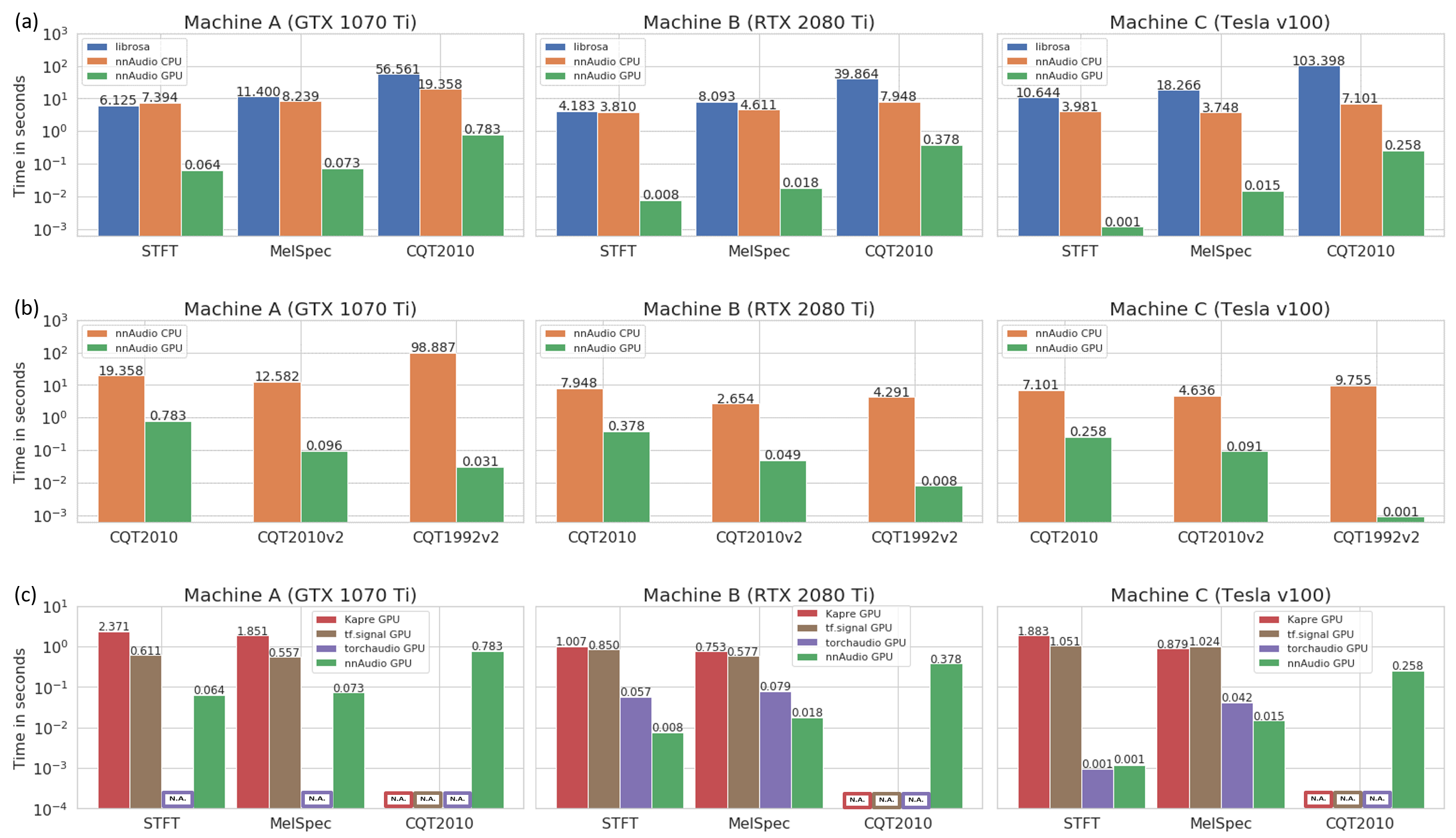
Speed
The speed test is conducted using three different machines, and it shows that nnAudio running on GPU is faster than most of the existing libraries.
Machine A: Windows Desktop with CPU: Intel Core i7-8700 @ 3.20GHz and GeForce GTX 1070 Ti 8Gb GPU
Machine B: Linux Desktop with CPU: AMD Ryzen 7 PRO 3700 and 1 GeForce RTX 2080 Ti 11Gb GPU
Machine C: DGX station with CPU: Intel Xeon E5-2698 v4 @ 2.20GHz and Tesla v100 32Gb GPU
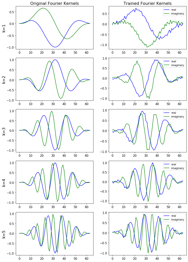
Trainable kernals
Fourier basis in STFT() can be set trainable by using trainable=True argument. Fourier basis in MelSpectrogram() can be also set trainable by using trainable_STFT=True, and Mel filter banks can be set trainable using trainable_mel=False argument. The same goes for CQT().
The follow demonstrations are avaliable on Google colab.
The figure below shows the STFT basis before and after training.
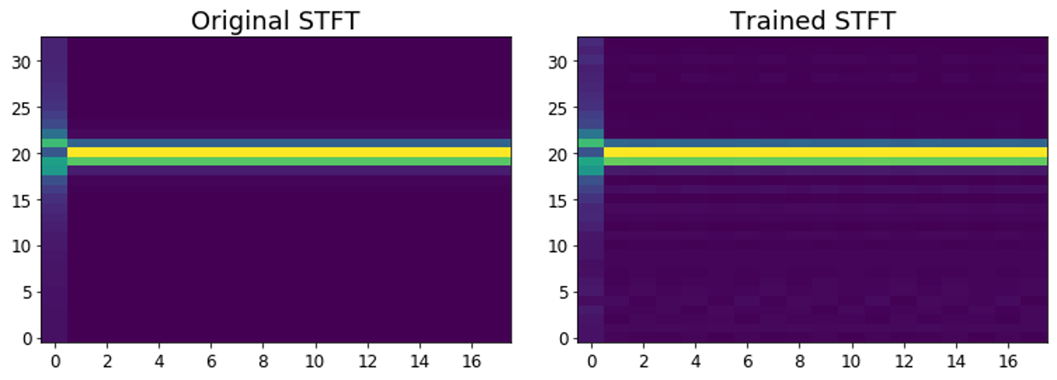
The figure below shows how is the STFT output affected by the changes in STFT basis. Notice the subtle signal in the background for the trained STFT.
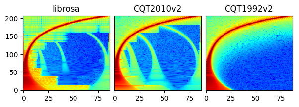
Different CQT versions
The result for CQT1992 is smoother than CQT2010 and librosa.
Since librosa and CQT2010 are using the same algorithm (downsampling approach as mentioned in this paper),
you can see similar artifacts as a result of downsampling.
For CQT1992v2 and CQT2010v2, the CQT is computed directly in the time domain
without the need of transforming both input waveforms and the CQT kernels to the frequency domain.
making it faster than the original CQT proposed in 1992.
The default CQT in nnAudio is the CQT1992v2 version.
For more detail, please refer to our paper
All versions of CQT are available for users to choose. To explicitly choose which CQT to use, you can refer to the CQT API section.